Two Roads to the Same bigram: Counting and Gradient Descent
The clever design of this episode: the same bigram model, implemented two ways — first by counting, then trained as a neural network — and the two turn out to agree almost exactly.
That comparison answers a question that has been hanging over the whole series: what is a neural network actually learning?
Road one: counting
The data, and what a bigram is
32,033 real English names, the shortest 2 letters and the longest 15.
bigram = bi (two) + gram (unit), one of the n-gram family:
| Name | Looks back | emma splits into |
|---|---|---|
| unigram | 0 | e, m, m, a |
| bigram | 1 | em, mm, ma |
| trigram | 2 | emm, mma |
The standard way to split:
chs = ['.'] + list(w) + ['.']for ch1, ch2 in zip(chs, chs[1:]): ...zip(chs, chs[1:]) is the standard sliding-window idiom — pair a list with a copy of itself offset by one.
Why no stray empty pair appears at the end:
ziptruncates to the shorter one. Here that is exactly what is wanted — the end marker appears only as an answer, never as an input. The very same behaviour was a hazard back in part 5’sNeuron.__call__(a wrong input length raises nothing).
Why start and end collapse into a single .
With two separate markers the table would be 28×28. But a start marker only ever appears at the beginning, so it is never a “next character”; an end marker only ever appears at the end, so it is never a “current character”. That leaves an entire row and an entire column permanently zero.
Collapsing them into one . compresses the table to 27×27 with no all-zero rows or columns. . takes index 0, so the letters start at 1:
stoi = {s: i+1 for i, s in enumerate(chars)}stoi['.'] = 0itos = {i: s for s, i in stoi.items()}The variable order differs between the two comprehensions, dictated by the data source:
enumerateyields(index, value)so it isfor i, s;items()yields(key, value)so it isfor s, i. Getting it backwards raises nothing and produces entirely wrong results.
A tensor, for the first time
N = torch.zeros((27, 27), dtype=torch.int32)for w in words: chs = ['.'] + list(w) + ['.'] for ch1, ch2 in zip(chs, chs[1:]): N[stoi[ch1], stoi[ch2]] += 1One object holding 729 numbers, rather than 729 Value objects — the point where scalar thinking gives way to tensor thinking.
Why not a dictionary: a dictionary can hold the data, but it cannot do wholesale arithmetic (normalising would need a loop) and cannot be visualised.
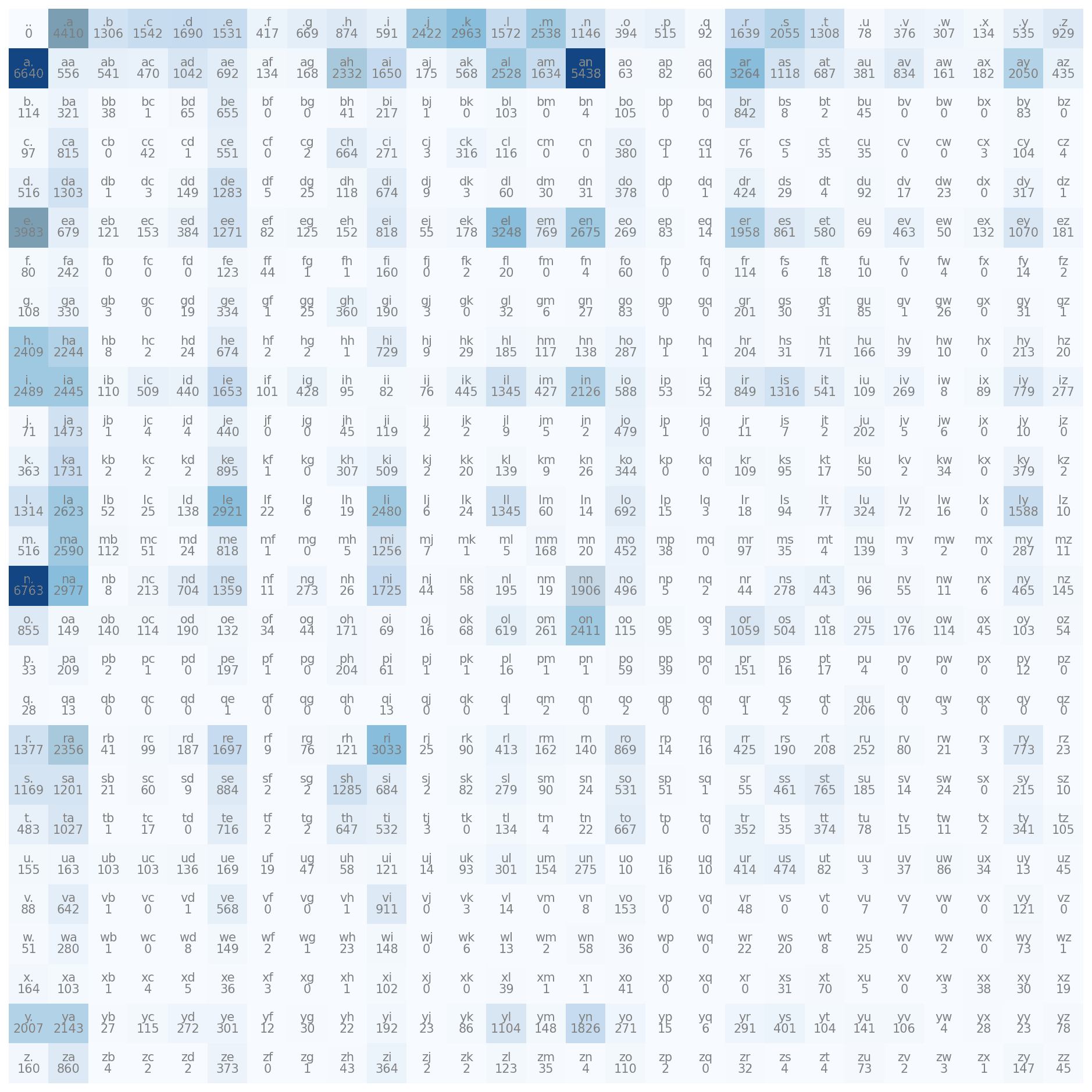
What can be read straight off it:
| Where | Meaning | What shows up |
|---|---|---|
Column 0 (x → .) | what names end in | n. 6763, a. 6640, e. 3983 |
Row 0 (. → x) | what names start with | .a 4410, .k 2963, .m 2538 |
| The darkest cells | frequent pairs | an 5438, ar 3264, el 3248 |
The whole q row | almost entirely white | only qu = 206, the rest near zero |
.. top left | 0 | empty names do not exist |
729 combinations are possible; 627 actually occur — 102 are missing. Those 102 zeros become a real problem shortly.
Sampling: the model makes something
g = torch.Generator().manual_seed(2147483647)ix = torch.multinomial(p, num_samples=1, replacement=True, generator=g).item()multinomial works like a roulette wheel: lay the probabilities out along a line where each segment’s length is that item’s probability, draw a uniform random number in 0–1, and see which segment it lands in. Longer segments get hit more often.
Written by hand it is just:
def pick(p, r): cum = 0.0 for i, prob in enumerate(p): cum += prob if r < cum: return iThe random number is the only source of uncertainty. Given
pandrthe answer is fully determined — there is no second roll. So with a fixed seed, a rerun produces exactly the same names. The chain is: seed fixed → sequence of r fixed → every draw fixed → names fixed.
Why not take the maximum: p.argmax() always returns the same thing, so the model would produce one name, and in an infinite loop at that. Drawing is what creates variety — and it is why GPT answers differently each time.
The generation loop:
ix = 0 # start from .while True: p = P[ix] # look up row ix ix = torch.multinomial(p, 1, generator=g).item() if ix == 0: break # drew a . — stop out.append(itos[ix])ix updating itself is the same move as x = layer(x) in part 5’s MLP.__call__ — one step’s output becomes the next step’s input.
The results: cexze, momasurailezitynn, konimittain, llayn, ka.
They look like names without being names. Against a uniformly random hjqzxvbn, bigram is short-sighted but has clearly learned something. The quality is limited because it only sees one character back — when generating that middle m in momasurai, the model has no idea what came before. That is the price of a context of 1.
Broadcasting and keepdim: the biggest trap here
P = N.float()P /= P.sum(1, keepdim=True)dim names the dimension that gets eliminated, which is counterintuitive:
| Written | Eliminates | Resulting shape | Intuitively |
|---|---|---|---|
A.sum(0) | dimension 0 (rows) | (3,) | the sum of each column |
A.sum(1) | dimension 1 (columns) | (3,) | the sum of each row |
keepdim is keep dimension — whether the summed dimension stays (with length 1). The numbers are identical; only the shape differs: A.sum(1) is (2,), A.sum(1, keepdim=True) is (2, 1).
Broadcasting aligns from the right, and copies along whichever dimension is 1. For a 3×3 example with row sums 10, 100, 10:
The correct (3,1) is a column, copied horizontally, so each row is divided by its own row sum → every row sums to 1.0 ✓
The wrong (3,) gets a 1 prepended to become (1,3) — a row, copied vertically, so every column is divided by the same number → the rows sum to 0.91, 8.2, 0.73 ✗
The essence of the error is that the denominator’s index changes from i to j:
correct: P[i][j] = N[i][j] / rowsum[i]wrong: P[i][j] = N[i][j] / rowsum[j]This bug raises nothing.
(3,3)and(3,)happen to broadcast successfully, so PyTorch assumes that is what was meant. The only defence is the habit of checking:print(P.sum(1))must be all 1.0.
While here, the three kinds of “multiplication”: A * B is element-wise (matching positions), A @ B is matrix multiplication (rows times columns, summed), and A.sum(dim) is a reduction (summing along a dimension and eliminating it). PyTorch’s / is not matrix division in the mathematical sense (that would be multiplying by an inverse) but element-wise division; broadcasting only pads the shapes, and the operation underneath stays element-wise.
loss = 2.4544
The three steps derived in the previous part, applied:
log_likelihood += torch.log(prob) # step 1: product becomes a sumnll = -log_likelihood # step 2: negateprint(nll / n) # step 3: divide by sample count → 2.4544Why the logarithm is unavoidable: multiplying 228,146 numbers below 1 gives roughly 10⁻²⁹⁶⁰⁰⁰, and the floating-point floor is 10⁻³⁰⁸ — it becomes 0 outright.
Why divide by N, three reasons: a total of 560,000 says only that there are many samples, nothing about model quality; datasets of different sizes need to be comparable; and the gradient then does not swing wildly with batch size, so the learning rate need not follow.
Translated into perplexity:
| Model | loss | Effectively guessing among |
|---|---|---|
| Pure chance | log 27 = 3.30 | 27 |
| bigram | 2.4544 | 11.6 |
| The MLP coming next | about 2.2 | about 9 |
| Ideal | 0 | 1 |
Loss falls linearly; the candidate count falls exponentially. From 3.30 to 2.45 is a drop of only 0.85, yet the candidates go from 27 to 11.6 — more than halved. The instinct is useful later: 2.0 → 1.5 (7.4 → 4.5 candidates) is a large improvement; 0.5 → 0.45 (1.65 → 1.57) is a small one. The same 0.05 means entirely different things in different ranges.
bigram cannot get lower because it only sees one character back. After q, the next character is almost certainly u (effectively one candidate); after a, many characters are plausible (effectively 15). 2.45 is the average over all positions.
model smoothing: those 102 zeros
Try a pair the dataset never contains: jq never occurs, its probability is 0, log 0 = -inf, and the loss becomes infinite. This is the practical consequence of the previous part’s log plot dropping vertically as x approaches 0.
The fix is to add k to every count:
P = (N + k).float()P /= P.sum(1, keepdim=True)| k | loss | Effective candidates | Notes |
|---|---|---|---|
| 0 | lowest | — | most accurate, but risks inf |
| 1 | 2.4544 | 11.6 | the compromise actually used |
| 10 | 2.51 | 12.3 | starts flattening the patterns |
| 100 | 2.69 | 14.7 | clearly worse |
| 1000 | 2.95 | 19.1 | approaching random |
Larger k is worse because genuinely frequent pairs get pushed down and rare ones pulled up, flattening the distribution. As k goes to infinity every probability becomes 1/27 and the loss approaches 3.30.
This is regularisation in embryo. k controls how much to trust the data versus how much room to leave: small k fits the training data exactly and may overfit; large k constrains the model from being too confident, trading training loss for generalisation.
jqnever occurring does not mean it is impossible — k=1 amounts to saying “assume every combination was seen once”. Later it turns out that L2 regularisation in a neural network and this+kare mathematically the same thing.
Road two: a neural network
Counting has already produced a working language model. Now rebuild it with a neural network and gradient descent.
Why bother, for three reasons: scale — counting three characters back needs a 27⁴-cell table, ten needs 27¹¹, and neither can ever be filled; flexibility — counting can only count, whereas a network can add activations, layers, different structures; and the thing this episode sets out to show — that on something as simple as bigram the two approaches agree almost exactly, so a neural network is not magic.
Building a training set: from iterating to sample pairs
Counting just iterates over the names. A network needs explicit (input, label) pairs:
xs, ys = [], []for w in words: chs = ['.'] + list(w) + ['.'] for ch1, ch2 in zip(chs, chs[1:]): xs.append(stoi[ch1]) ys.append(stoi[ch2])xs = torch.tensor(xs)ys = torch.tensor(ys)emma yields 5 samples: (., e), (e, m), (m, m), (m, a), (a, .) — as indices, (0,5), (5,13), (13,13), (13,1), (1,0).
These are the same bigrams counting iterated over, only stored explicitly as two tensors this time.
The
tensorversusTensortrap:torch.tensor([1,2,3])is int64 and stays integral;torch.Tensor([1,2,3])is float32 and forces floats. Lowercase is required here — indices must be integers, and floats cannot subscript.
one-hot and a single-layer network
xenc = F.one_hot(xs, num_classes=27).float() # (N, 27)W = torch.randn((27, 27), generator=g)logits = xenc @ W # (N,27) @ (27,27) = (N,27)No hidden layer, no bias, no activation — one matrix multiplication. This is the smallest possible neural network. Shape-wise, that middle 27 is what gets eliminated.
W has the same dimensions as counting’s 27×27 table — which is no coincidence.
Two arguments that must be written out:
num_classes=27, since otherwise PyTorch infers the width from the largest value present; and.float(), sinceone_hotreturns int64 and the next step multiplies against float weights.Also,
@is matrix multiplication (rows times columns, summed) while*is element-wise — entirely different operations.
one-hot times a matrix ≡ a table lookup
xenc[0] is [1,0,0,…,0], and multiplied by W:
[1,0,0,…] @ W = 1×W_row0 + 0×W_row1 + … = W_row0The other 26 rows are all multiplied away by 0. Check it: torch.allclose(logits[0], W[xs[0]]) → True.
This is the motivation for embeddings. With a 50,000-word vocabulary, one-hot is a 50,000-dimensional vector and the multiplication costs 50,000 multiplies (49,999 of them by zero) — where a lookup costs one index. Not an optimisation trick; a necessity.
The same reasoning already appeared in the previous part’s cross-entropy:
probs[target]is equivalent to multiplying by a one-hot vector and summing, minus 26 multiplications by zero. The two are the same fact.
softmax: structurally compared with counting
counts = logits.exp() # step 1: make them positiveprobs = counts / counts.sum(1, keepdim=True) # step 2: normalisekeepdim=True again — for the same reason as when normalising N earlier.
Read counts as “the counts the model believes in”:
| Counting | Neural network | |
|---|---|---|
| Counts | N (integers, counted) | logits.exp() (positives, computed) |
| Probabilities | N / N.sum(1, keepdim) | counts / counts.sum(1, keepdim) |
The normalisation step is identical; only the origin of the counts differs. What exp does is precisely turn an arbitrary real number into a legal count — counts must be positive, and logits can be either sign.
What training does: adjust
Wuntil the computed counts approach the counted ones.
Computing the loss: there is no “expected probability” to compare against
The true answer is not a probability distribution but one definite character. In the dataset, emma’s e is followed by m — not “70% likely to be m”.
So the comparison is not subtracting two distributions, but one lookup and one logarithm:
y = ys[i] # the correct index, say 13p = probs[i, y] # pull column 13 out of that rowloss = -torch.log(p)| What the truth is | How to compare | |
|---|---|---|
| Squared error (V1) | a number | subtract, then square |
| Cross-entropy (V2) | a class | look up that class’s probability, take −log |
A feel for the numbers (assuming the correct answer is m):
| The model’s distribution | probs[i,13] | loss |
|---|---|---|
evenly spread, [0.037]*27 | 0.037 | 3.30 |
wrong bet: a:0.9, m:0.01 | 0.01 | 4.61 |
right bet: m:0.9 | 0.90 | 0.11 |
The middle row fares worst — because it was confidently wrong. That is precisely cross-entropy’s design intent.
The batched form uses advanced indexing to pull out every correct entry at once:
loss = -probs[torch.arange(N), ys].log().mean()torch.arange(N) is [0,1,2,…], paired positionally with ys, equivalent to probs[0, ys[0]], probs[1, ys[1]], and so on. Two index tensors of equal length, paired by position, with no loop.
A useful health check:
Wis randomly initialised, so the initial loss should sit near log(number of classes) — 3.30 here (in practice slightly higher, around 3.5–4, since a randomWproduces some meaningless preferences). Wildly higher usually means an initialisation problem: the weights are too large and the model starts out confidently talking nonsense.
The training loop: identical to V1
for k in range(300):    xenc = F.one_hot(xs, num_classes=27).float()    logits = xenc @ W    counts = logits.exp()    probs = counts / counts.sum(1, keepdim=True)    loss = -probs[torch.arange(num), ys].log().mean()
W.grad = None # zero loss.backward() W.data += -50 * W.grad # update| Part 6, written by hand | PyTorch |
|---|---|
for p in n.parameters(): p.grad = 0.0 | W.grad = None |
loss.backward() | loss.backward() |
p.data += -0.05 * p.grad | W.data += -50 * W.grad |
Three details:
requires_grad=True— tensors do not track gradients by default and it has to be switched on. This is the_prev/_backwardwritten by hand in part 4, built into PyTorchW.grad = Nonerather than= 0— setting it toNoneis more efficient in PyTorch, since the backward pass then assigns rather than accumulatesW.datarather thanW—.databypasses gradient tracking, so this update does not itself get recorded into the graph
Why the learning rate is 50 (part 6 used 0.05, a thousand times smaller): the gradient is averaged over 228,146 samples, which dilutes it; and a single linear layer has a gentle loss surface, so large steps do not oscillate.
The two roads meet
| Counting | Neural network | |
|---|---|---|
| Parameters | 27×27 count table N | 27×27 weights W |
| Contents | counts (non-negative integers) | logits (any real number) |
| How obtained | counted | trained by gradient descent |
| To probabilities | divide by row sums | exp first, then divide by row sums |
| loss | 2.4544 | about 2.46 |
The probability tables can be compared directly:
Pcount = (N + 1).float(); Pcount /= Pcount.sum(1, keepdim=True)with torch.no_grad(): Pnet = (torch.eye(27) @ W).exp() Pnet = Pnet / Pnet.sum(1, keepdim=True)print('largest difference:', (Pcount - Pnet).abs().max().item())torch.eye(27) is the identity matrix, every row of which is a one-hot vector, giving all 27 rows of logits in one go.
This answers what a neural network is actually learning: it is approximating the statistics of the data.
And there is something here that is exceptionally rare in real projects: counting supplies this task’s theoretical optimum. The network matched it, which means training is genuinely finished rather than “could use more epochs”.
So why use a neural network at all
| Context | Cells in the table | Counting |
|---|---|---|
| 1 character | 27² = 729 | countable; 627 actually occur |
| 3 characters | 27⁴ = 531,441 | 228,146 samples cannot fill it |
| 5 characters | 27⁶ ≈ 390 million | most cells are 0 |
| 10 characters | 27¹¹ ≈ 5.6×10¹⁵ | out of the question |
No amount of data fills that table. An unseen combination has probability 0, so the model declares it impossible — no generalisation whatsoever.
A neural network handles any context with a fixed parameter count. That is its entire value.
Sampling strategy is a dial
The network gives 27 probabilities and multinomial draws one; only together do they produce the next character. The model is saying “after a, n is 20% likely and . is 18%”, not “it will be n” — because the data itself is varied.
The results: junide, janasah, prelay, kohin, tolian. The specific names differ from counting’s (the probability tables differ in the later decimals, and drawing amplifies that), but the style matches: similar length distribution, alternating vowels and consonants, familiar endings.
| Strategy | How | Effect |
|---|---|---|
| greedy | take the maximum | deterministic, conservative, repetitive |
| temperature | divide logits by T before softmax | small T conservative, large T divergent |
| top-k | draw only among the top k | excludes low-probability oddities |
| top-p | draw within cumulative probability p | dynamic cut-off |
Pᵢ = e^(zᵢ/T) / Σⱼ e^(zⱼ/T)That temperature parameter in the API is this. It reshapes the probability distribution rather than the random number.
A model’s output is a distribution, not an answer. Getting from distribution to answer is sampling, which is separate and adjustable. The same model behaves very differently under different strategies.
smoothing is L2 regularisation
loss = -probs[torch.arange(num), ys].log().mean() + 0.01 * (W**2).mean()# └────────── data term ──────────┘ └─ regulariser ─┘The two terms pull in opposite directions: the data term wants W to fit the data, which needs large weights to separate frequent from rare; the regulariser wants W near 0 regardless of what the data says. λ decides which has the louder voice.
Why “W → 0” means “a uniform distribution”:
W = 0 → logits = [0,…,0] → exp → [1,…,1] → normalise → [1/27, …]Perfectly uniform — nothing learned at all. So:
| In the limit | Result | |
|---|---|---|
| smoothing | k → ∞ | counts flattened → uniform |
| L2 | λ → ∞ | W all zero → uniform |
Both pull the distribution towards uniform, differing only in what they act on — one the counts, the other the weights.
The gradient makes it clearer. The regulariser’s derivative with respect to W is 2λ/729 · W, so each update multiplies W by a number slightly below 1. That operation is called weight decay, and PyTorch’s optimisers have a parameter by that name.
It is unconditional: whatever the data says, every round pulls a little towards 0. Only patterns that recur can resist that pull; incidental noise cannot — which is the mechanism by which it improves generalisation.
What “trained enough” means
A loss of 0 is neither achievable nor desirable in a language model — it would mean every position is 100% certain, whereas a really can be followed by n, . or r. That is the data’s inherent uncertainty, not a defect in the model.
Three criteria: below the random baseline of 3.30, so something was learned; close to the known level for comparable models, and bigram’s ceiling is 2.45; and the loss curve flattening, so another thousand rounds changes nothing.
More important is the validation set — the moment validation loss bottoms out and turns up is the moment to stop. There is nothing to worry about here: 729 parameters against 228,146 samples means the model has no capacity to memorise. But parameter counts grow sharply from here, and then this criterion becomes essential.
The same bigram model: counting gives 2.4544, gradient descent gives 2.46. Two entirely different roads, almost the same destination — a neural network is not magic, it is approximating the statistics of the data. Its value is not being more accurate but being able to scale.
That completes V2. New tools acquired: tensors and broadcasting, the keepdim trap, advanced indexing, multinomial sampling, softmax, cross-entropy, and PyTorch’s requires_grad / backward / .data.
Next is V3: the context widens from 1 character to 3, and the loss falls from 2.45 to about 2.2. It introduces embeddings properly (the direct application of today’s “multiplication is a lookup”), hidden layers, mini-batch training, and the split into training, validation and test sets.