Divide the Learning Rate by 3: Four Plots That Turn Guessing into Arithmetic
Part 16 closed by saying that BatchNorm had knocked out the top two levels of part 14’s diagnostic
checklist: σ_W can be off by a factor of a thousand and it no longer matters, and saturation gets
pulled back on the spot. So what is left of the checklist?
Push it down one level. The first two steps are automatic now, and what actually needs looking at is the three plots below them — plus a fourth that produces the one directly actionable step in the entire diagnostic flow.
Where the four plots come from
The four plots are not four separate pieces of code — the first three read three things left behind
by one and the same forward-backward pass, and the fourth is recorded all the way through training.
So the place to start is where those things come from: the previous code could hand over none of
them, because forward returned only the logits and h and z were thrown away as soon as they were
computed. Refactor first, and only then is there anything to plot.
First, reshape the network
Part 5 already wrote this shape once. Back then it was Neuron / Layer / MLP built on Value:
self.layers = [...], for layer in self.layers: x = layer(x), and a parameters() that flattens
each layer’s parameters upward. This time the same shape is rebuilt on matrices — it is not a new
idea.
Three classes, each responsible for exactly three things:
| method | what it does | why it is needed |
|---|---|---|
__init__ | create and hold its own parameters | every layer minds its own things |
__call__ | the forward pass, storing the result in self.out | so layer(x) is directly callable; all four plots read that out |
parameters() | report which parameters it owns | one line outside collects all of them |
Part 5 already covered __call__: b(5) is syntactic sugar for b.__call__(5), and PyTorch’s
nn.Module overloads it too. What is new here is one word that did not come up then — Tanh has
no parameters at all, and still has to implement parameters():
class Tanh: def parameters(self): return []So that the line outside needs no special case:
parameters = [C] + [p for layer in layers for p in layer.parameters()]This is duck typing: Python does not care what class you are, only what you can do. Implement
__call__ and parameters() and you can go into layers. A uniform interface is what lets the
collection be one line.
What the network looks like
⚠️ This network’s
n_hiddenis 100, not the 200 of parts 14 through 16. Those three were about a two-layer30 → 200 → 27network; this one is six layers of 100. The shapes(30,100) / (100,100) / (100,27)are the only ones that add up to 47,024 parameters.
Two adjustments at initialisation:
with torch.no_grad(): layers[-1].gamma *= 0.1 # squash the output layer → initial loss ≈ ln(27) for layer in layers[:-1]: if isinstance(layer, Linear): layer.weight *= 5/3 # tanh's gainThe first line is part 14’s “fix the initial loss”, just applied somewhere else: it used to be
W2 * 0.01, and now that the last layer is a BN, it is that layer’s γ instead.
The second line explains something that looks like an oversight until you think about it —
why gain is not written into Linear.__init__. The class divides by √fan_in and nothing
more; gain is multiplied in when the network is assembled. Different activations have different
gains (5/3 for tanh, √2 for ReLU), and a class has no business assuming what comes after it.
Only the two halves together make up the full σ_W = gain / √fan_in.
Which tensor each plot reads
| plot | reads | recorded when | shape |
|---|---|---|---|
| ① forward activations | layer.out, the five Tanh layers | the diagnostic cell’s forward pass | (32, 100) |
| ② backward gradients | layer.out.grad, the same five | the same backward pass | (32, 100) |
| ③ parameter gradients | p.grad, seven 2-D tensors | the same backward pass | (30,100), (100,100)… |
| ④ update/data | ud, appended every training step | the whole run | 20,000 steps × one row each |
The first three are three cross-sections of a single forward-backward pass — which is why they have to be produced in one cell, with nothing else in between. The fourth is different: it has to be recorded inside the training loop as it goes.
with torch.no_grad(): ud.append([((lr*p.grad).std() / p.data.std()).log10().item() for p in parameters])The layer.out field is exactly what the refactor above bought — without it the first two plots
cannot be drawn at all.
❗ A trap first: evaluate wipes out layer.out
To begin with, layer.out.grad is None everywhere, and this line is why:
print(f"train {evaluate(Xtr,Ytr):.4f} val {evaluate(Xdev,Ydev):.4f}")evaluate runs another forward pass internally, overwriting every layer.out — and that pass
happens inside @torch.no_grad(), so the tensors it produces are not in the computation graph and
will never have a .grad.
This is built into the self.out design: it always holds the most recent forward pass, and
anything that calls forward in between wipes it. PyTorch works around this with hooks; this is the
stripped-down version.
The fix is to run diagnostics in their own cell, with no retain_grad() in the training loop
(it would be overwritten anyway, and would waste memory in the meantime):
ix = torch.randint(0, Xtr.shape[0], (batch_size,))loss = F.cross_entropy(forward(Xtr[ix]), Ytr[ix])
for p in parameters:    p.grad = Nonefor layer in layers:    layer.out.retain_grad()      # ← has to come before backwardloss.backward()
Plot immediately after that cell, and do not call evaluate in between.
Why retain_grad() is needed at all: parameter gradients like W1.grad are kept by default,
while intermediate gradients like ∂L/∂h are discarded as soon as they are used — nobody ever
writes h.data += -lr * h.grad, so they exist only as the route to ∂L/∂W1. Part 13 used this
switch once, to print an intermediate gradient and check a backward pass by hand. It is 3B1B’s
baton: it updates nothing itself,
but the next layer needs it to keep moving backwards.
❗ no_grad and training=False are two different things
Part 11 used @torch.no_grad() to write evaluate, and there was no BN in the network then, so it
was not a problem. Now there is, and the two switches have to be kept apart:
| what it controls | |
|---|---|
torch.no_grad() | whether the computation graph is recorded — saves memory and time, does not change the numbers |
layer.training = False | whether BN uses the current batch’s statistics or the running ones — changes the result directly |
Evaluation needs both. Writing no_grad without switching training leaves BN normalising with
the validation set’s own statistics — the model gets to peek at the validation distribution, and
the result comes out optimistic.
What the run gives
parameters 47024   layers 17     0/20000  loss 3.3298      ← the initial loss is already at ln(27) = 3.2958  5000/20000  loss 2.2419 10000/20000  loss 2.1913 15000/20000  loss 2.1039
train 2.1339   val 2.1531      40.8 seconds
No hockey stick — the model starts from honest ignorance rather than spending its first few hundred steps undoing an initialisation mistake. The steep opening drop from part 14’s curve is simply absent this time.
| model | layers | steps | val |
|---|---|---|---|
| hand-tuned 0.2 | 2 | 130,000 | 2.0994 |
| BN + running | 2 | 130,000 | 2.1106 |
| 6 layers + BN | 6 | 20,000 | 2.1531 |
Six layers comes out worse — but on 6.5× fewer steps, and the loss was still falling at step
15,000. The point of this section is not the score, it is the structure. With layer.out in
place, the four plots become drawable.
Plot ①: forward activations
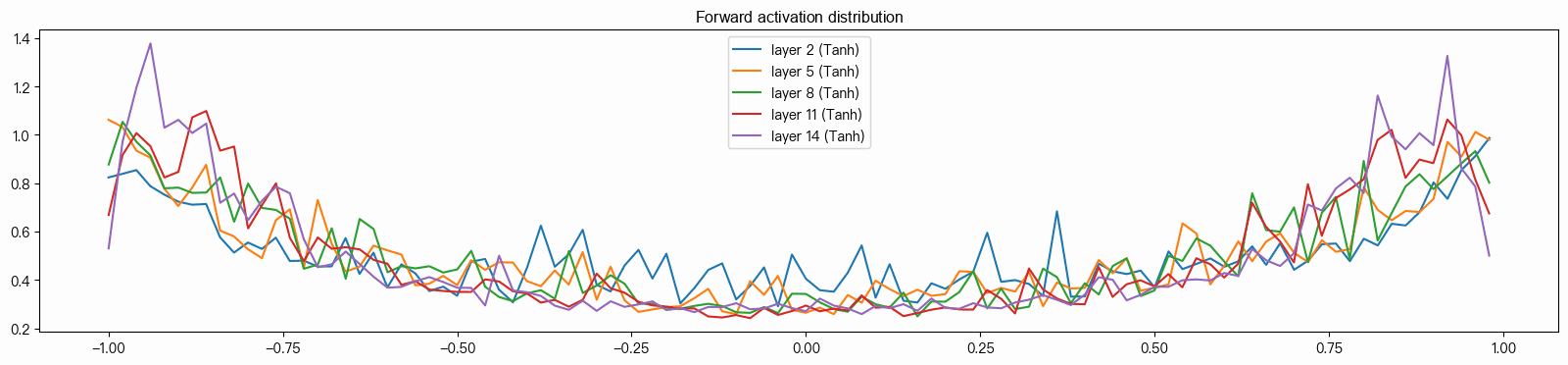
What is drawn is the output h of the five Tanh layers. The horizontal axis is the value of h
(pinned to −1…1 by tanh itself), and the vertical axis is density.
Why density rather than counts: the five layers are meant to be overlaid and compared. If one layer
had a different width, plotting counts would make it sit lower automatically, and the comparison
would be about layer size rather than distribution shape. Density = count ÷ (total × bin width),
so the area is always 1. Converting: 3200 values, bins of 0.04, 160 in one bin → density
160 / (3200 × 0.04) = 1.25.
Read the numbers first, then the plot
layer 2 (Tanh): mean +0.00 std 0.64 saturated 5.4%layer 5 (Tanh): mean -0.01 std 0.66 saturated 6.2%layer 8 (Tanh): mean -0.01 std 0.67 saturated 5.4%layer 11 (Tanh): mean +0.00 std 0.68 saturated 4.3%layer 14 (Tanh): mean -0.01 std 0.69 saturated 3.5%These five lines reach the conclusion faster than the plot does. Each column answers one thing:
mean is where the centre sits (should be ≈ 0), std is how spread out it is
(staying flat across layers matters most), and saturated is what fraction has stopped learning
(1–10% is healthy).
The means being 0 is BatchNorm’s doing. tanh is an odd function, so a mean sitting off in the positive half means only half of it is in use — and BN’s very first step forces the centre back to zero. That ±0.01 is sampling noise.
⚠️ The per-layer ratio is 1.019, not 1.08
0.64 → 0.66 → 0.67 → 0.68 → 0.69 is a cumulative rise of 8% over five layers. That number
is right.
But five values have only four transitions between them, so the per-layer ratio is
(0.69/0.64)^(1/4) = 1.019, not 1.08. Extrapolating with 1.08 gives 48× at 50 layers;
with 1.019 it gives 2.6×:
| per-layer ratio | after 20 | after 30 | after 50 |
|---|---|---|---|
| 0.6 | 3.7e−5 | 2.2e−7 | signal gone |
| 1.019 (measured) | 1.46 | 1.76 | 2.56 |
| 1.5 | 3325 | 1.9e5 | blown up |
The conclusion is unchanged — one glance at the std column tells you whether this architecture
can be stacked deep, and the answer is still yes. But the number has to be right, because plot ②
is about to be compared against it.
⚠️ This batch of numbers uses a threshold of 0.97
Saturation is computed like this:
saturated = (t.abs() > 0.97).float().mean() * 100The threshold is a human choice. Part 14’s numbers used 0.99; this section of Karpathy’s
switches to a stricter 0.97. atanh(0.97) = 2.092 while atanh(0.99) = 2.647 — same model,
different ruler, different number. So the 5.4% here cannot be compared directly against any
saturation figure in part 14.
Where the threshold goes at all is a question about how much gradient is left:
| |h| | 1 − h² | gradient remaining |
|---|---|---|
| 0 | 1.000 | 100% |
| 0.9 | 0.190 | 19% |
| 0.97 | 0.059 | 5.9% |
| 0.99 | 0.020 | 2% |
❗ Less saturation is not automatically better
The left panel is the one that matters: 0% saturated, and yet σ_h / σ_z = 0.96 — over that
range tanh is very nearly the identity function. Six layers stacked that way are equivalent to a
single matrix multiply, and the depth bought nothing. Seeing 0%, go back and check std; do not
assume lower is better. This is also why Kaiming targets σ = 1 rather than “as small as
possible”.
The middle panel’s σ_z = 1.10 gives σ_h = 0.655 and 5.7% saturated, which lines up with the
measured σ_h ≈ 0.65 and 5.4%.
The U shape itself is not a disease; it is what tanh inevitably does:
range of z | width | maps to h | width |
|---|---|---|---|
| −0.5 to 0.5 | 1.0 | −0.46 to 0.46 | 0.92 |
| 2 to 3 | 1.0 | 0.964 to 0.995 | 0.031 |
Large z values get squeezed into a short stretch of h near ±1, where the density is naturally
high. What matters is how deep the U runs (the three multipliers below were measured off
histogram bins, which is not the same quantity as the analytic fractions in the plot above — do not
put them side by side):
| version | ends / middle | saturated |
|---|---|---|
| V4 as it started | ~50× | 62.3% |
| hand-tuned 0.2 | ~2.5× | 1.4% |
| now | ~4× | ~5% |
Two statements worth keeping apart
“5.4% of the activations are saturated” is correct. “5.4% of the neurons are dead” is not. The same neuron produces different outputs for different samples — it may be saturated on sample A and perfectly normal on B. What is genuinely dead is what saturates for every sample:
dead = (h.abs() > 0.97).all(0) # True all the way down the sample axisPlot ②: backward gradients
It differs from plot ① by exactly one word:
t = layer.out.grad # plot ① was layer.outThe thing this plot gets stuck on is
layer.out.gradcoming backNoneeverywhere — that trap and its fix are covered above under “Where the four plots come from”: run the diagnostics in their own cell.
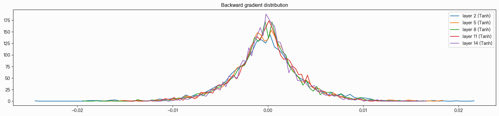
The shape is a bell, not a U
This is the biggest visual difference between the two plots, and the reason is direct: gradients have no bound. They are free real numbers, not compressed by tanh, and they are sums of many terms — the central limit theorem hands you a normal shape. The spike near 0 says most positions need only a small adjustment and a few need a large one, which is normal.
The horizontal ranges differ by a factor of 100 as well: −1 to 1 for plot ①, −0.02 to 0.02 for plot ②. Gradients are just small numbers.
What the run gives
layer 2 (Tanh): mean -0.000000 std 4.116130e-03layer 5 (Tanh): mean +0.000000 std 3.720852e-03layer 8 (Tanh): mean -0.000000 std 3.545590e-03layer 11 (Tanh): mean +0.000000 std 3.342206e-03layer 14 (Tanh): mean +0.000000 std 3.152745e-03All five sit at e-03, and the largest is only 1.3× the smallest. For contrast, vanishing gradients
put a factor of 100,000 between the two ends.
Note that the direction has flipped: backpropagation runs from the loss forwards, so it starts at
layer 14 (3.15e−3) and ends at layer 2 (4.12e−3). The per-layer ratio is
(4.12/3.15)^(1/4) = 1.069.
The means are exactly 0, more thoroughly than plot ①’s ±0.01 — gradients are symmetric in sign, with
some samples wanting a neuron turned up and others wanting it turned down, and the two cancel. A
mean clearly off zero would say every sample wants to push the same way, which usually means there
is still a lot of room to improve (early training looks like that).
⚠️ Both directions are healthy, but they are not “nearly the same”
| per-layer ratio | after 20 | after 30 | after 50 | |
|---|---|---|---|---|
| forward (plot ①) | 1.019 | ×1.46 | ×1.76 | ×2.56 |
| backward (plot ②) | 1.069 | ×3.79 | ×7.39 | ×28.0 |
Neither blows up nor vanishes, and “this six-layer network could be stacked to 20–30 layers” holds. But forward drifts 1.9% per layer and backward drifts 6.9% — backward drifts 3.6× as fast — and calling the two directions “nearly identical” compares a five-layer cumulative 8% against a per-layer 6.9%.
Why plot ② matters more than plot ①
| what decay costs | recoverable? | |
|---|---|---|
| forward signal | later layers receive a weaker signal | yes — a later layer can amplify it back |
| backward gradient | earlier layers receive no update signal | no — unlearnable is unlearnable |
Vanishing gradients mean the first few layers’ parameters stay at their initial values forever. That is the direct reason deep networks would not train before 2015, and it is the problem residual connections, mentioned back in part 12, were built to solve.
Plot ③: parameter gradients
The first two plots draw a layer’s intermediate result; this one draws the gradient of the
parameters themselves — p.grad, the thing actually used for the update:
p.data += -lr * p.grad.
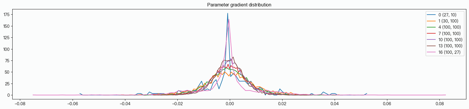
❗ This is the one plot of the four where the numbers beat the picture. What is drawn is the distribution of gradient values, while what this section is actually about is
grad/data— the gradient’s std divided by the parameter’s own std. That quantity is not on the plot; it is in the printed column. The picture’s one job here is to show youC’s spike.
Why the seven indices skip around
The code only picks the two-dimensional ones:
if p.ndim == 2: # weight matrices only| index | shape | which one |
|---|---|---|
| 0 | (27, 10) | the embedding table C |
| 1 | (30, 100) | layer 1’s Linear |
| 2, 3 | (100,) | layer 1’s BN γ and β ← skipped |
| 4, 7, 10, 13 | (100, 100) | layers 2–5’s Linear |
| 16 | (100, 27) | the output Linear |
A stride of 3 = one Linear weight plus two BN parameters. γ and β are skipped because they are one-dimensional and on a different scale; mixing them in would only muddle the picture.
❗ Read grad/data, not std
ratio = σ(gradient) / σ(the parameter itself)Read it as: roughly what percentage of itself does this tensor get changed by, each step.
weight (27, 10) | std 1.194477e-02 | ratio 1.183552e-02weight (30, 100) | std 9.806189e-03 | ratio 2.992686e-02weight (100,100) | std 7.715235e-03 | ratio 4.201583e-02weight (100,100) | std 6.782562e-03 | ratio 3.722516e-02weight (100,100) | std 6.164674e-03 | ratio 3.422855e-02weight (100,100) | std 5.627475e-03 | ratio 3.148335e-02weight (100, 27) | std 1.065568e-02 | ratio 5.203685e-02By gradient std, C is the largest. By ratio, C is the smallest. The two give opposite
conclusions. That is the whole reason for dividing — an absolute change means nothing, a relative
rate of change means something.
The middle four are strikingly even: 4.20 → 3.72 → 3.42 → 3.15 (×10⁻²). The four (100,100) layers
are on exactly the same scale; none of them is racing ahead or stalling.
Both ends deviate, for different reasons
Back out each tensor’s own std from ratio = gradient std ÷ parameter std, and the two ends
explain themselves:
| ratio | implied parameter std | gradient std | |
|---|---|---|---|
C, low | 1.18e−2 | 1.009 | 1.19e−2 (largest) |
| the middle four | ~3.5e−2 | ~0.181 | ~6e−3 |
| output layer, high | 5.20e−2 | 0.205 | 1.07e−2 |
C has the smallest ratio, and the denominator is the main reason: C comes from an unscaled
randn, so its own std ≈ 1.0, 5.5× that of the middle layers, while its gradient is only
about 2× larger. Divide and it lands lowest. Gradient sparsity — a batch only touches some of the
27 rows, leaving a lot of exact zeros — is what keeps the numerator from growing further. That is
part 13’s Jacobian of nothing but 0s and 1s: ∂L/∂C is non-zero only on the rows that were used.
⚠️ At the output-layer end, the first reason given in the notes does not hold. The notes say it was “squashed by
gamma *= 0.1, so the denominator is small”. But backing the number out, the output layer’s ownstdis 0.205 — the largest of the six weight matrices, not the smallest.gamma *= 0.1squashes BN’s γ, not the Linear’s weight. Its ratio is high because the numerator is high: a gradientstdof 1.07e−2, 1.89× that of the layer next to it. The second reason is the real one: it sits closest to the loss, so its gradient is naturally stronger.
What pathology looks like: a layer whose ratio is 100× smaller barely learns; 100× larger may oscillate and diverge; a steady decline across layers is the parameter-side version of vanishing gradients, and then the thing to fix is plot ②, not the learning rate.
⚠️ But plot ③ is a snapshot of one step. Any one of twenty thousand steps could be atypical.
Plot ④: update/data
The first three are snapshots; this one is the trajectory of the whole training run — the most useful of the four.
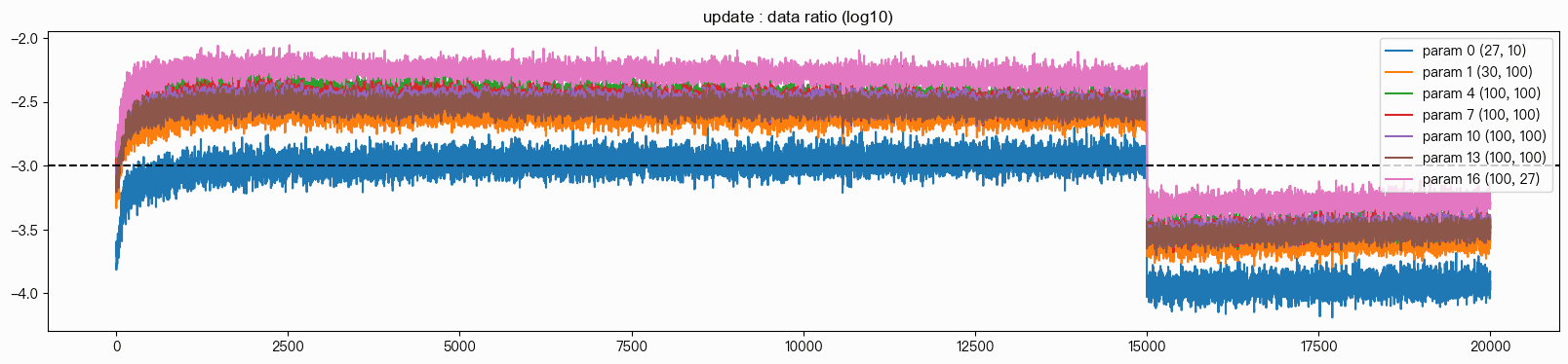
One thing only the picture shows: all seven are bands, not lines. Every step draws a fresh mini-batch, so the ratio jitters, and the thickness of each band is that jitter. It is a diagnostic signal in its own right — the cheat sheet’s “the band suddenly widens = lr too large” is about this thickness, and here it never widens.
What each quantity in the formula is
y = log10( σ(lr × grad) / σ(data) )Take W1: the parameter’s own std ≈ 0.33, this step’s gradient std ≈ 9.8e−3, multiplied by
lr = 0.1 for an actual change of ≈ 9.8e−4, a ratio of 0.30%, which in log10 is −2.52.
Why divide by data: “changed by 0.001” means nothing on its own; what matters is how big that
is relative to the parameter itself.
parameter std | change | ratio | verdict |
|---|---|---|---|
| 0.30 | 0.001 | 0.33% | ✅ |
| 0.001 | 0.001 | 100% | ❌ doubles in a step, about to blow up |
| 100 | 0.001 | 0.0001% | ❌ ten thousand steps to move 1% |
Why take log10: three reasons, and the last one is the point. Across several orders of magnitude
a linear axis crushes 0.0001, 0.001 and 0.01 together; the rule-of-thumb 1e-3 becomes a whole
number, so axhline(-3) just works; and multiplication becomes addition — lr ÷ 10 is a clean
drop of exactly 1. This is the same idea as part 11’s logarithmic sweep: ratios become equal
spacing on a log axis.
Four phases
| phase | position | explanation |
|---|---|---|
| steps 0–2500 | climbing from about −3.8 to −2.5 | the initial gamma *= 0.1 squashed the output and the gradients with it; as the model starts learning, the ratio climbs to its steady level. On the plot almost all of this happens in the first few hundred steps; the rest is a slow drift into place |
| 2500–15000 | steady at −2.5 | ✅ flat |
| step 15000 | a clean 1.0 drop | lr goes from 0.1 to 0.01 |
| 15000–20000 | steady at −3.5 | ⚠️ too low |
Where the seven lines sit before the decay: output layer at −2.35, the middle four at −2.4 to −2.5,
the first layer at −2.6, and C at −2.95, sitting right on the baseline.
Plot ④ is plot ③ multiplied by lr
That claim can be checked directly. Multiply plot ③’s ratios by lr = 0.1 and take log10:
| parameter | implied by plot ③ | actual position in plot ④ |
|---|---|---|
C | −2.93 | −2.95 |
| first layer | −2.52 | −2.60 |
| the middle four | −2.38 … −2.50 | −2.4 to −2.5 |
| output layer | −2.28 | −2.35 |
Every row lines up, with a maximum discrepancy of 0.08 — and given that plot ③ is one step while plot ④ is a whole stretch, a gap of that size is exactly what should be there. The spread between the seven lines comes entirely from the denominator, which is the same thing plot ③’s ratios were showing.
Three levels of judgement: trend > position > spread
Trend first. A climb followed by a plateau, or a plateau throughout, is ✅. A persistent upward drift means parameters are shrinking or gradients are growing, and it is heading for trouble; a persistent sink means learning is stalling; a sudden jump that is not a learning-rate decay means something is wrong.
Then position, relative to the −3 baseline:
| deviation | factor | verdict | multiply lr by |
|---|---|---|---|
| within ±0.3 | 0.5–2× | ✅ ideal | leave it |
| ±0.3–0.7 | 2–5× | acceptable (this run) | optional tweak |
| 0.7–1.5 high | 5–30× | ⚠️ too large | ÷ 10^(deviation) |
| 0.7–1.5 low | 5–30× | ⚠️ too small | × 10^(deviation) |
| beyond ±1.5 | 30×+ | ❌ definitely wrong | go back and check plots ① and ② |
Spread last. Here it runs from −2.35 to −2.95, a spread of 0.60, under a factor of 10 —
healthy. Beyond 2 (a factor of 100) the fix is that layer’s initialisation, not the global
learning rate.
Filling in the gap part 11 left
When part 11 covered logarithmic learning-rate sweeps, it ended on a hard limitation: “its value is in ruling out, not in picking a winner.” The U-shaped curve carries history dependence, and narrowing the range from ×1000 to ×40 is as far as it goes.
update/data picks up exactly there:
new lr = old lr × 10^(−3 − current position)Currently at −2.5, targeting −3, that comes out as × 10^(−0.5) = ÷ 3.2.
Guessing becomes arithmetic. The sweep does the coarse pass; this ratio does the fine one.
What this plot tells you to do
The first three are green, and the fourth is the only one that hands over an action: the early stretch sits 0.5 too high, and the decay spans too much.
lr = 0.05 if step < 15000 else 0.02 # both stretches land closer to -3# or decay smoothlylr = 0.1 * (0.1 ** (step / max_steps))Sitting at −3.5 after the decay means each step changes the parameters by about
10^(−3.5) ≈ 0.032%, against 10^(−2.5) ≈ 0.32% before it — the last 5,000 steps do roughly what
500 earlier steps would have done. That is why the loss barely moves over that final stretch:
cutting 0.1 straight to 0.01 is too big a jump.
🔑 This is what the toolkit is supposed to look like: it does not tell you whether the model is good, it tells you what to change next.
The diagnostic handbook
With all four plots read, here is the whole thing compressed onto one page, to look up while tuning:
Neural-network diagnostic handbook · the four plots at a glance
When a model will not converge, work down this list. Until the level above is fixed, the level below reports numbers you cannot trust.
❗ The order cannot be reversed — bad initialisation disguises itself as “wrong learning rate”, and a wrong learning rate disguises itself as “not enough capacity”
| symptom | diagnosis | prescription |
|---|---|---|
| std shrinking layer by layer (0.6→0.1) | signal decay | raise gain, or add BN |
| std growing layer by layer | signal amplification | lower gain |
| std stable (ratio 0.9–1.1) | ✓ healthy | — |
| saturation > 30% | many neurons cannot learn | shrink the weights, or add BN |
| saturation 1–10% | ✓ healthy | — |
| saturation ≈ 0% with a small std | ❗ degenerated into linear; depth wasted | raise gain |
| mean clearly off 0 | skewed; only half of tanh in use | add BN / check BN is running |
Whether the threshold is 0.97 or 0.99 is a human choice — just keep it consistent when comparing
| symptom | diagnosis | prescription |
|---|---|---|
| all layers at e-03, ratio < 2 | ✓ gradients get through | — |
| first layer 100×+ smaller than last | ✗ vanishing gradients | add BN / adjust gain / residuals |
| first layer 100×+ larger than last | ✗ exploding gradients | lower gain / clip gradients |
| one layer falls off a cliff | that layer has a problem | check its initialisation and activation |
| all None | no retain_grad, or evaluate wiped it | run diagnostics in their own cell |
❗ The direction is last layer → first layer. When it decays, the first layer has the smallest std. ※ This is the most important one: forward decay can be amplified back later, but a gradient that never arrives cannot be learned from at all
| symptom | diagnosis | prescription |
|---|---|---|
| middle layers on one order of magnitude | ✓ learning speed is even | — |
| one layer 100× smaller | that layer barely learns | check if its parameters are too large |
| one layer 100× larger | may oscillate and diverge | check if its parameters are too small |
| a steady decline across layers | the parameter-side vanishing gradient | go back and fix plot ❷ first |
| embedding C: low ratio, spiked histogram | large parameters + sparse gradients | ignore |
| output layer: high ratio | it sits closest to the loss | ignore |
Why not std: different layers hold parameters on different scales — dividing is what makes the rate of change comparable
| symptom | diagnosis | prescription |
|---|---|---|
| climb, then a plateau | ✓ normal | — |
| flat throughout | ✓ normal | — |
| drifting upward | ✗ parameters shrinking or gradients growing | lower lr / add weight decay |
| sinking steadily | ✗ learning has stalled | raise lr / check for saturation |
| the band suddenly widens | ❗ lr too large | lower lr |
| a clean drop of ∆ at the decay point | ✓ it took effect, ∆ = log10(decay factor) | — |
| falls below −3.5 after the decay | ❗ decay spans too much; the tail is wasted | use a smaller decay factor |
| still at −2.5 after the decay | the decay was too small to matter | use a larger decay factor |
| deviation | factor | verdict | multiply lr by |
|---|---|---|---|
| within ±0.3 | 0.5–2× | ✓ ideal | leave it |
| ±0.3–0.7 | 2–5× | acceptable | optional tweak |
| 0.7–1.5 high | 5–30× | ❗ too large | lr ÷ 10^deviation |
| 0.7–1.5 low | 5–30× | ❗ too small | lr × 10^deviation |
| beyond ±1.5 | 30×+ | ✗ definitely wrong | check plots ❶❷ first |
new lr = old lr × 10^( −3 − current position )e.g. −2.5 → ÷ 3.2
| < 1 (10×) | ✓ healthy | ||
|---|---|---|---|
| 1–2 | ❗ uneven — check those layers’ initialisation | ||
| > 2 (100×) | ✗ fix that layer, not the global lr | ||
the first three plots must be green firstwith vanishing gradients plot ❹ sits below −5 — tuning lr there does nothing at all
−3 is not a law−3 for SGD on a small network; Adam may sit at −2.5; fine-tuning is usually around −4
the final standard is val lossall four green and val still not falling → the problem is capacity or data, not the training process
ix = torch.randint(0, Xtr.shape[0], (batch_size,))
loss = F.cross_entropy(forward(Xtr[ix]), Ytr[ix])
for p in parameters: p.grad = None
for layer in layers: layer.out.retain_grad()
loss.backward()
with torch.no_grad():
    ud.append([((lr*p.grad).std() / p.data.std()).log10().item()
               for p in parameters])
The flow across the top of that poster is part 14’s diagnostic order, so it is not re-explained here. What follows takes the plots one at a time and fills in what part 14 did not have: what to look at in each individual plot.
Plot ①, forward activations
Three numbers: std, saturated, mean.
| symptom | diagnosis | prescription |
|---|---|---|
std shrinking layer by layer (0.6→0.1, say) | signal decay | raise gain, or add BN |
std growing layer by layer | signal amplification | lower gain |
std stable (ratio 0.9–1.1) | ✅ | — |
| saturation > 30% | many neurons cannot learn | shrink the weights, or add BN |
| saturation 1–10% | ✅ | — |
saturation ≈ 0% with a small std | ⚠️ degenerated into linear; the depth is wasted | raise gain |
mean clearly off 0 | skewed distribution; only half of tanh is in use | add BN, or check whether BN is actually running |
Plot ②, backward gradients
One thing only: are the five std values on the same order of magnitude? The direction is
layer 14 → layer 2, so if it is decaying, the first layer (layer 2) has the smallest std.
| symptom | diagnosis | prescription |
|---|---|---|
all layers at e-03, ratio < 2 | ✅ gradients get through | — |
| layer 2 more than 100× smaller than layer 14 | ❌ vanishing gradients | add BN / adjust gain / add residual connections |
| layer 2 100× larger than layer 14 | ❌ exploding gradients | lower gain / clip gradients |
| one layer falls off a cliff | that layer has a problem | check that layer’s initialisation and activation |
all None | retain_grad() was not called, or evaluate wiped it | run diagnostics in their own cell |
Plot ③, parameter gradients
Read the grad/data column only; ignore std.
| symptom | diagnosis | prescription |
|---|---|---|
| middle layers on the same order | ✅ learning speed is even | — |
| one layer 100× smaller | that layer barely learns | check whether its parameters are too large |
| one layer 100× larger | may oscillate and diverge | check whether its parameters are too small |
| a steady decline across layers | the parameter-side version of vanishing gradients | go back and fix plot ② |
Two deviations that can be ignored: the embedding table C sits low with a spike in its histogram
(large parameters plus sparse gradients), and the output layer sits high (it is closest to the loss).
Plot ④, update/data
Three levels by priority: trend > position > spread, with the three tables above. What is left is the decay check:
| symptom | meaning |
|---|---|
| a clean drop of ∆ at the decay point | ✅ it took effect, ∆ = log10(the decay factor) |
| falls below −3.5 after the decay | ⚠️ the decay spans too much; the tail of the run is wasted |
| still at −2.5 after the decay | the decay was too small to matter |
❗ Three things that have to be remembered
| premise | why |
|---|---|
| the first three plots must be green first | with vanishing gradients, plot ④ sits below −5, and tuning lr does nothing there |
| −3 is not a law | −3 for SGD on a small network; Adam may sit at −2.5; fine-tuning is usually around −4 |
| the final standard is still val loss | all four green and val still not falling → the problem is capacity or data, not anything these four plots measure |
Code worth copying
Diagnostic setup, its own cell, plot immediately after:
ix = torch.randint(0, Xtr.shape[0], (batch_size,))loss = F.cross_entropy(forward(Xtr[ix]), Ytr[ix])for p in parameters: p.grad = Nonefor layer in layers: layer.out.retain_grad()loss.backward()Recording ud during training (plot ④ needs it):
with torch.no_grad(): ud.append([((lr*p.grad).std() / p.data.std()).log10().item() for p in parameters])All four sets of numbers in one pass, no plotting:
print("—— plot ① forward activations ——")for i, l in enumerate(layers[:-1]):    if isinstance(l, Tanh):        t = l.out        print(f"  {i:>2} std {t.std():.3f}  saturated {(t.abs()>0.97).float().mean()*100:.1f}%")
print("—— plot ② backward gradients ——")for i, l in enumerate(layers[:-1]):    if isinstance(l, Tanh):        print(f"  {i:>2} std {l.out.grad.std():e}")
print("—— plot ③ parameter gradients ——")for p in parameters:    if p.ndim == 2:        print(f"  {str(tuple(p.shape)):<12} ratio {p.grad.std()/p.std():e}")
print("—— plot ④ update/data ——")for i, p in enumerate(parameters):    if p.ndim == 2:        print(f"  param {i:>2} last step {ud[-1][i]:+.2f}")
Two things not done yet
That closes out V4. Two comparison runs are still outstanding, recorded here as they are, with no conclusions filled in for them:
- rerun with
gainset to 0.5 and see what the four plots look like when things are unhealthy — so far only the healthy version has been seen, and without a contrast there is no real reading skill to speak of - retune the learning rate as plot ④ suggests (
0.05 / 0.02) and see whether val drops below 2.1531 — that is what actually cashes in the phrase “computed, not guessed”
From part 14 to this one, V4’s four parts have been four faces of the same thing: first knowing what to measure (the three metrics), then knowing how to make it hold automatically (BatchNorm), and finally knowing how to read a measurement as an action.
The value of the first three plots is that they make the fourth trustworthy — when the gradients are not even arriving, tuning the learning rate is tuning a problem that does not exist.